A Selection of My Favorite Graphs

Hypocycloid and Zeros

In my complex analysis research, we used winding numbers to count the number of zeros of complex-valued harmonic functions. This animation shows the image of the critical curve side-by-side with the plot of the zeros and critical curve so that one can see the close relationship between winding numbers and zeros. The animation shows an example from the subfamily studied in Section 5 of Applying the Argument Principle to Count Zeros of Harmonic Functions with Poles.

Hypocycloid Animation

For my 2022 talk on zeros of complex-valued harmonic polynomials, I animated the geometric construction of a hypocycloid using two circles.

Cuspidal projections of products of Eisenstein series

At the close of the 2021 Clemson University REU, my group gave several talks to the other REUs that Clemson was hosting and then to REUs hosted by other universities in a virtual conference. In preparing for my presentation with William Frendreiss, I created a visual representation of the bounds that we proved for the n = 2 case of our theorem. We proved that for large enough weight k, the coefficients a_f(n) of E_k² - E_2k do not satisfy the required Hecke eigenform relation, so E_k² - E_2k cannot be an eigenform. If E_k² - E_2k was an eigenform, then equality between the blue and the red dots would hold for every weight k, but we see that it only holds for small weights when it is forced to by dimension considerations.

Zeros of a Family of Complex-Valued Harmonic Trinomials

This diagram was used to prove that the self-intersections of the hypocycloid were located at an angle that we could explicitly write. I love how clean and tidy the end result turned out.

Non-convex geometry of numbers and continued fractions

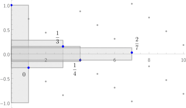
This first picture is the graph that is displayed in the paper. This displays the algorithm running for α = 3 - e with p = 0.5. You can see that two convergents are skipped in a row.

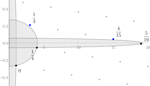
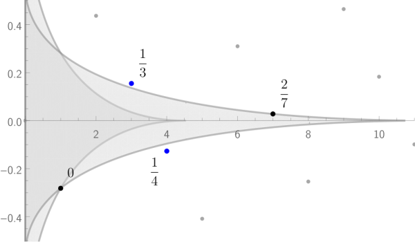
With Zach Hacking, I gave a talk on this paper in February 2021. These are three of my favorite graphs from the talk. These show the difference in what points the algorithm picks up for different p values. All three are for α = 3 - e, with the first being the infinity norm, the second is p = 2, and the last is p = 0.5.